Creating Australian census data choropleth map with geopandas

5 min readFeb 1, 2022

The Australian census could provide interesting insight into demographic data for the area you are living in or planning to move. This data is available from the Australian Bureau of Statistics (ABS) free of change. It can also be a good data source for practising data visualisation.

In this article, I would like to show you how to download this data and create a choropleth map for almost any metric available in 2016 Census data.

Census data packs

The ABS DataPacks download page provides a form where you can select which census data to download. There are two files we need.

First one is a ZIP file with census data. It’s available for the whole country and for each state. Metadata contains descriptions for each census metric. First column specifies in which CSV file this metric is located. second is column name. In our example CSV file name G02 (2016Census_G02_NSW_SSC.csv) and column is Median_tot_fam_inc_weekly.

Metadata_2016_GCP_DataPack.xlsx contains description for each census metric

CSV file contains actual values for each statistical area. SSC10001 is a unique key identifying each suburb in Australia. Median_tot_fam_inc_weekly column contains “Median total family income ($/weekly)” for this suburb.

Second file ZIP file contains geographical shapes for statistical areas, such as suburbs in out case. It is saved as an ESRI Shapefile format which we can read into GeoDataFrame using geopandas.

Preparation

We need to install pandas and geopandas libraries using pip

!pip install pandas geopandas

Import required libraries

import pandas as pd
import geopandas as gpd
import zipfile
import requests
import io

And set some configuration variables:

# SA1-SA4 - statistical areas
# SSC - suburbs
geography_type = "SSC"# Australian state
au_state = "NSW"# metric to display
census_metric = "Median_tot_fam_inc_weekly"# location to zoom in for detail map
zoom_radius_center ="Sydney GPO"
zoom_radius_meters = 30000# census data files on ABS website
shapes_url = f"https://www.censusdata.abs.gov.au/CensusOutput/copsubdatapacks.nsf/All%20docs%20by%20catNo/Boundaries_2016_{geography_type}/$File/2016_{geography_type}_shape.zip"
data_url = f"https://www.censusdata.abs.gov.au/CensusOutput/copsubdatapacks.nsf/All%20docs%20by%20catNo/2016_GCP_{geography_type}_for_{au_state}/$File/2016_GCP_{geography_type}_for_{au_state}_short-header.zip"# location keys 
geography_type_fields = { 
    "SA1": { "geo_key": "SA1_7DIGIT", "data_key": "SA1_7DIGITCODE_2016" },
    "SA2": { "geo_key": "SA2_7DIGIT", "data_key": "SA2_7DIGITCODE_2016" },
    "SA3": { "geo_key": "SA3_7DIGIT", "data_key": "SA3_7DIGITCODE_2016" },
    "SA4": { "geo_key": "SA4_CODE", "data_key": "SA4_CODE_2016" },
    "SSC": { "geo_key": "SSC_CODE", "data_key": "SSC_CODE_2016" },
}
geo_key = geography_type_fields[geography_type]["geo_key"]
data_key = geography_type_fields[geography_type]["data_key"]

shapes_url and data_url contain URL of ABS Census data pack files for given state and geography type. Since each geography type data pack uses different keys for statistical areas (SSC, SA1-SA4) I’ve defined these column names in the dictionary.

zoom_radius_center and zoom_radius_meters specify area and radius which I would like to zoom into when generating a choropleth map.

Loading statistical area shapes into GeoDataFrame

I will download geographical shapes ZIP file from ABS webserver and load data into GeoDataFrame directly

shapes_gpd = gpd.read_file(shapes_url)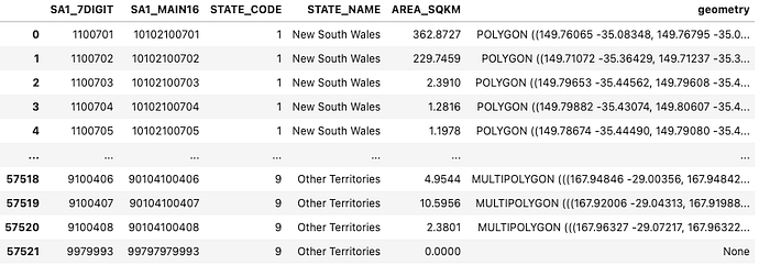

shapes_gpd contains geometry for each statistical area

Geometry column contains Polygon or Multipolygon objects defining area shape. You can plot these polygons using the plot() method of GeoDataFrame. Y axis shows latitude and X axis longitude.

shapes_gpd.plot()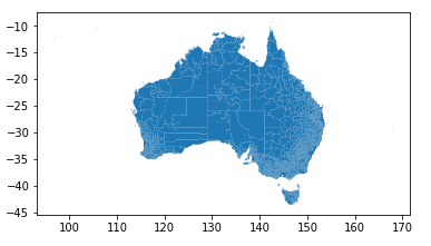

Just like pandas DataFrame, we can filter GeoDataFrame by Australian state:

shapes_gpd[shapes_gpd.STATE_NAME == "New South Wales"].plot()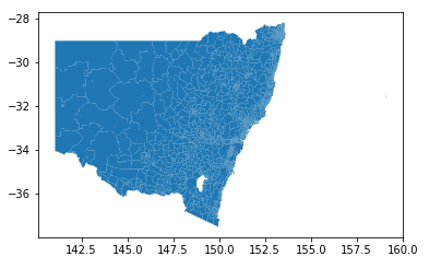

Statistical area polygons located in New South Wales

Loading census metrics

Load census metrics ZIP file from ABS server:

response = requests.get(data_url)
data_zipfile = zipfile.ZipFile(io.BytesIO(response.content))

Since the ZIP archive contains more than 50 CSV files with various metrics, I will filter file list using regular expression “.*2016Census_G02” and load that file into DataFrame. After that I will merge it with geo data frame containing statistical area shapes:

import re
nsw_ssc_df = shapes_gpd.rename(columns={geo_key: data_key})
for zipinfo in data_zipfile.filelist:
    if re.match(r".*2016Census_G02", zipinfo.filename):
        print(zipinfo.filename)
        census_data_df = pd.read_csv(data_zipfile.open(zipinfo.filename), dtype={data_key: 'str'})
        print(nsw_ssc_df.columns)
        census_df = pd.merge(nsw_ssc_df, census_data_df)
        
census_gdf = gpd.GeoDataFrame(census_df, geometry=nsw_ssc_df.geometry)
census_gdf

Now census_gdf geo dataframe contains both geoshapes and census metrics:

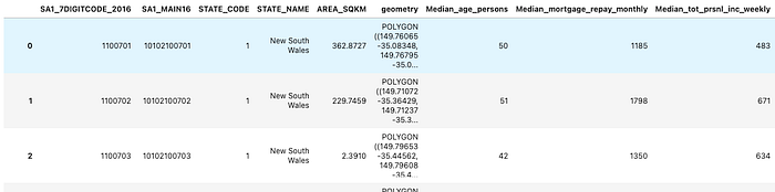
Now a choropleth map with selected metric can be generated. Legend on right hand side shows correlation between income value and statistical area colour

census_gdf.plot(census_metric, legend=True, figsize=(20,15), cmap="plasma")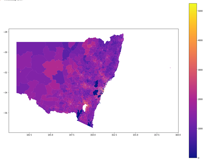

NSW map with Median_tot_fam_inc_weekly metric

Zoom in into the specified area

While seeing data for the whole NSW is exciting, it’s not very usable. Most likely you will be interested in the area where you live or plan to move. Let’s create a map with the centre at a given point and radius in metres from this point.

In my example I will set zoom_radius_center to ”Sydney GPO” (General Post Office) located in the Sydney CBD. geocode() will find geographical coordinates for this location.

sydney_gpo_df = gpd.tools.geocode([zoom_radius_center], provider='nominatim', user_agent="maksym demo")

Now we need to convert coordinates into map projection EPSG 20255 which uses metres instead of geographical coordinates, add buffer with radius in metres and convert it back into map projection EPSG 4283 which uses latitude and longitude.

sydney_gpo_radius_df = sydney_gpo_df.to_crs(epsg=20255).buffer(zoom_radius_meters).to_crs(epsg=4283)
sydney_gpo_radius_df.plot()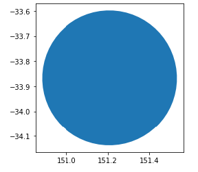

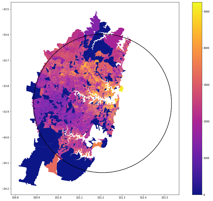
Geoshape representing 30 km radius from Sydney GPO

Next step is to apply filter to GeoDataFrame so only areas inside this circle shape will be returned

area_census_gdf = census_gdf[census_gdf.geometry.intersects(sydney_gpo_radius_df.iloc[0])]

Now we can plot both statistical areas data & zoom area circle as a map:

import matplotlib.pyplot as plt
fig, ax = plt.subplots(nrows = 1, ncols = 1, figsize=(20,15))area_census_gdf.plot(census_metric, ax=ax, legend=True, figsize=(20,15), cmap="plasma")
sydney_gpo_radius_df.plot(ax=ax, color="#00000000", edgecolor="black", linewidth=2)

Median total family income ($/weekly) for Sydney, NSW

Do you want to experiment with using another census metric or zoom into different areas? Go to complete code example on Colab and give it a try.

Complete example code is also available as a notebook on GitHub.